Global weed compendium network
This is a co-occurrence network I made from a weed species by geographic region list - an output from Rod Randall’s fantastic Global Weeds Compendium Randall (2017). This is not to be confused with CABI’s awesome Invasive Species Compendium. I contributed a few data sheets for CABI’s ISC a few years ago (Buddenhagen 2013a, b, 2014a, b, c, 2015, Buddenhagen 2016).
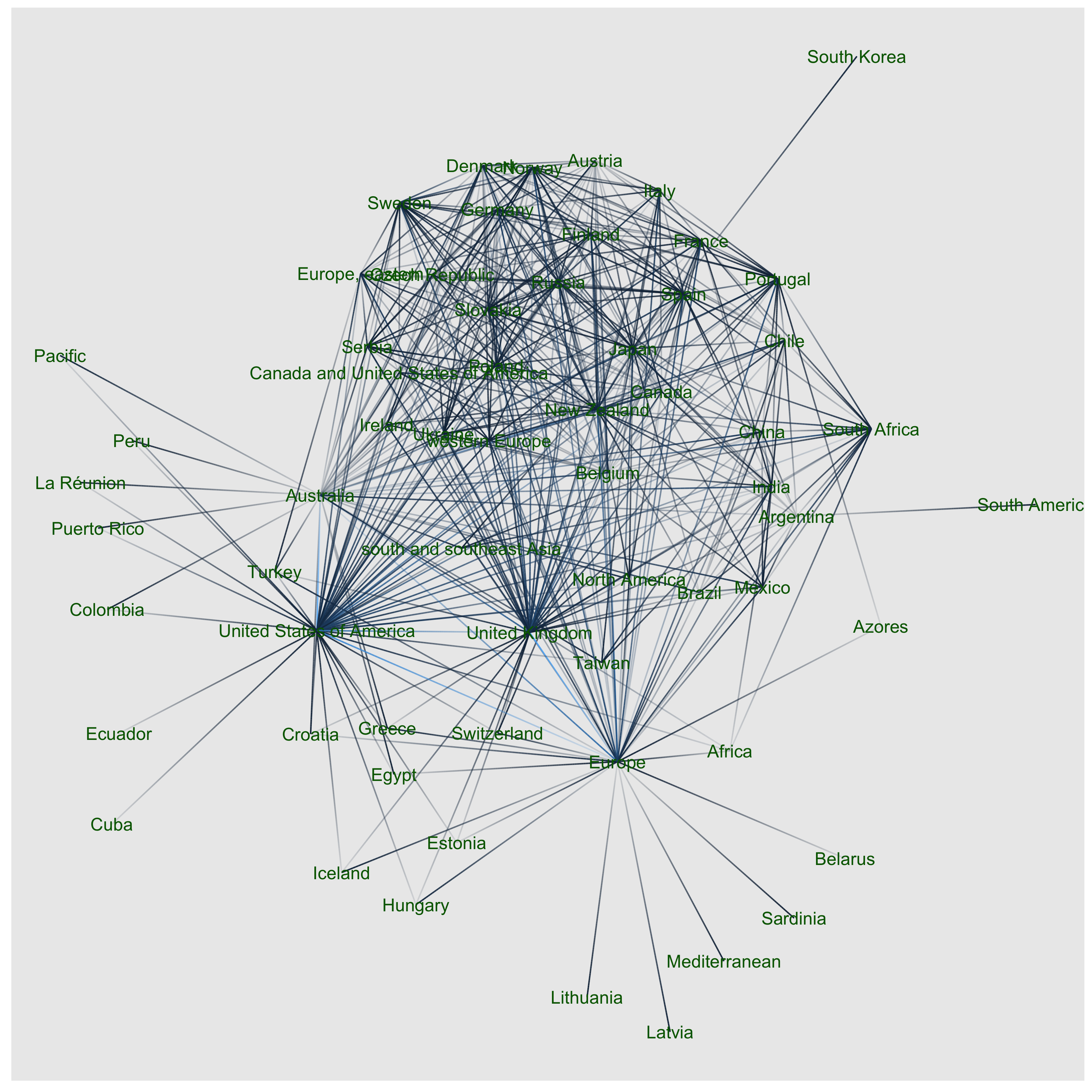
I used the igraph and ggraph packages to make the network Csardi & Nepusz (2006). This is much reduced by using only highly weighted links - otherwise its too huge because Randall’s dataset is big! I think this “stress” layout makes nodes means countries that share more species are closer together. Let’s compare the Australian and New Zealand location in the network topology. Here NZ is more similar to temperate Asian countries and Europe, while Australia shares species with drier Mediterranean climates, tropical America and Asia.
Code
library(tidyverse)
library(readxl)
library(ggraph)
library(igraph)
#read in data from Randall's compendium https://www.researchgate.net/project/Global-Weed-Country-Dataset-available
country_spp<-read_xlsx("Randall 2017 Global Compendium countries with species.xlsx")#make links
country_spp<-country_spp %>% rename("to"=`Full taxa name with author citation`) %>% rename("from"=`Compendium Country`) %>% select("from", "to")
#adjacency matrix country shared species
country_by_spp <- table(country_spp)
#make adjacency matrix
adjacency <- country_by_spp %*% t(country_by_spp)
diag(adjacency)<-0 #remove self loops#use igraph to make igraph object
g<-graph_from_adjacency_matrix(adjacency,weighted=T, mode="undirected")
#get attributes
attributes(V(g))#see which node is the NZ node.
V(g)$name=="New Zealand"#get reduced graph baed on edge weights
g_sub <- delete.edges(g, E(g)[weight <= max(weight)*.15]) #reduces links by link weight
g_sub <- delete.vertices(g_sub , which(degree(g_sub)==0)) #removes isolated nodes after links are removed#ggraph is a tidy implementation of igraph
ggraph(g_sub, layout = 'kk') +
geom_edge_fan(aes(colour = weight, alpha = stat(index))) +
geom_node_text(aes(label = name, size=1), colour="darkgreen")+
theme(legend.position="none")ggsave("country network.png", width=11, height=11)